The Double Pendulum System

This page gives an overview over the mathematical description of the double pendulum dynamics.

Equation of Motion

_images/schematic.png
\[\newcommand{\vect}[1]{\boldsymbol{#1}} \newcommand{\dvect}[1]{\dot{\boldsymbol{#1}}} \newcommand{\ddvect}[1]{\ddot{\boldsymbol{#1}}} \newcommand{\mat}[1]{\boldsymbol{#1}}\]

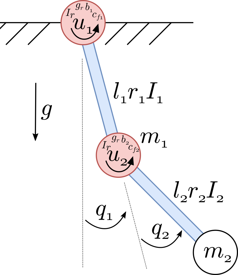
We model the dynamics of the double pendulum with 15 parameters which include 8 link parameters namely masses \((m_1, m_2)\), lengths \((l_1, l_2)\), center of masses \((r_1, r_2)\), inertias \((I_1, I_2)\) for the two links, and 6 actuator parameters namely motor inertia \(I_r\), gear ratio \(g_r\), coulomb friction \((c_{f1}, c_{f2})\), viscous friction \((b_1, b_2)\) for the two joints and gravity \(g\).

The generalized coordinates \(\vect{q} = (q_1, q_2)^T\) are the joint angles measured from the free hanging position. The state vector of the system contains the coordinates and their time derivatives: \(\vect{x} = (\vect{q}, \dvect{q})^T\). The torques applied by the actuators are \(\vect{u} = (u_1, u_2)\). The equations of motion for the dynamics of a dynamical system can be written as

\[\begin{split} \dvect{x} &= \vect{f}(\vect{x}, \vect{u}) \label{eq:dyn}\\ % \left[ \begin{matrix} % \dvect{q} \\ % \ddvect{q} % \end{matrix} \right] &= \left[ \begin{matrix} \dvect{q} \\ \mat{M}^{-1}(\mat{D} \vect{u} - \mat{C}(\vect{q}, \dot{\vect{q}}) \dot{\vect{q}} + \mat{G}(\vect{q}) - \mat{F}(\dot{\vect{q}})) \label{eq:dyn2} \end{matrix} \right]\end{split}\]

The equation in the bottom half of the vector is also known as manipulator equation. For the double pendulum, the entities in the manipulator equation are the mass matrix (with \(s_1 = \sin(q_1), c_1 = \cos(q_1), \ldots\))

\[\begin{split}\mat{M} = \left[ {\begin{array}{cc} I_1 + I_2 + l_1^2m_2 + 2l_1m_2r_2c_2 + g_r^2I_r + I_r & I_2 + l_1m_2r_2c_2 - g_rI_r \\ I_2 + l_1m_2r_2c_2 - g_rI_r & I_2 + g_r^2I_r \\ \end{array}} \right],\end{split}\]

the Coriolis matrix

\[\begin{split}\mat{C} = \left[\begin{matrix} - 2 \dot{q}_2 l_{1} m_{2} r_{2} s_2 & - \dot{q}_2 l_{1} m_{2} r_{2} s_2\\ \dot{q}_1 l_{1} m_{2} r_{2} s_2 & 0 \end{matrix}\right], \label{eq:coriolis_matrix}\end{split}\]

the gravity vector

\[\begin{split}\mat{G} = \left[\begin{matrix} - g m_{1} r_{1} s_1 - g m_{2} \left(l_{1} s_1 + r_{2} s_{1+2} \right)\\ - g m_{2} r_{2} s_{1+2} \end{matrix}\right], \label{eq:gravity_matrix}\end{split}\]

the friction vector

\[\begin{split}\mat{F} = \left[\begin{matrix} %b_1 \dot{q_1} + c_{f1} \text{sign}(\dot{q_1}) \\ %b_2 \dot{q_2} + c_{f2} \text{sign}(\dot{q_2}) b_1 \dot{q_1} + c_{f1} \arctan(100\,\dot{q_1}) \\ b_2 \dot{q_2} + c_{f2} \arctan(100\,\dot{q_2}) \end{matrix} \right] \label{eq:friction_matrix}\end{split}\]

(the \(\arctan(100\dot{q}_i)\) function is used to approximate the discrete step function for the coulomb friction)

and the actuator selection matrix \(\mat {D}\)

\[\begin{split}\mat{D}_{full} = \left[\begin{matrix} 1 & 0 \\ 0 & 1 \end{matrix} \right], \quad \mat{D}_{pendu} = \left[\begin{matrix} 1 & 0 \\ 0 & 0 \end{matrix} \right], \quad \mat{D}_{acro} = \left[\begin{matrix} 0 & 0 \\ 0 & 1 \end{matrix} \right]\end{split}\]

for the fully actuated system, the pendubot or the acrobot.

Energy

  • Kinetic Energy

\[E_{kin} = \dot{\vect{q}}^T \mat{M} \dot{\vect{q}}\]
  • Potential Energy

\[E_{pot} = - m_1 g r_1 c_1 - m_2 g (l_1 c_1 + r_2 c_{1+2}).\]
  • Total Energy

\[E = E_{kin} + E_{pot}\]

System Identification

\[\newcommand{\vect}[1]{\boldsymbol{#1}} \newcommand{\dvect}[1]{\dot{\boldsymbol{#1}}} \newcommand{\ddvect}[1]{\ddot{\boldsymbol{#1}}} \newcommand{\mat}[1]{\boldsymbol{#1}}\]

For the identification of the 15 model parameters, we fix the natural, provided and easily measurable parameters \(g, g_r, l_1\) and \(l_2\) and consider the independent model parameters

\[m_1 r_1,\, m_2 r_2,\, m_2,\, I_1,\, I_2,\, I_r,\, b_1,\, b_2,\, c_{f1},\, c_{f2}.\]

The goal is to identify the parmaters of the dynamic matrices in the manipulator equation

\[\mat{M} \ddot{\vect{q}} + \mat{C}(\vect{q}, \dot{\vect{q}}) \dot{\vect{q}} - \mat{G}(\vect{q}) + \mat{F}(\dot{\vect{q}}) - \mat{D} \vect{u} = 0\]

By executing excitation trajectories on the real hardware, data tuples of the form \((\vect{q}, \dot{\vect{q}}, \ddot{\vect{q}}, \vect{u})\) can be recorded. For finding the best system parameters, one can make use of the fact that the dynamics matrices \(\mat{M}, \mat{C}, \mat{G}\) and \(\mat{F}\) are linear in the independent model parameters and perform a least squares optimization for the dynamics equation on the recorded data.