The Physics of a Simple Pendulum

Equation of Motion

$$I\ddot{\theta }+b\dot{\theta }+c_f\text{sign}(\dot{\theta })+mgl\sin (\theta )=\tau$$

where

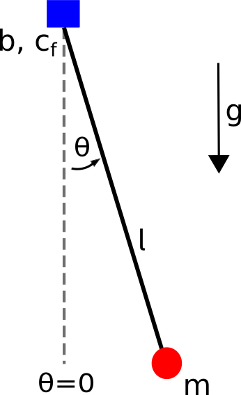
• $\theta$, $\dot{\theta }$, $\ddot{\theta }$ are the angular displacement, angular velocity and angular acceleration of the pendulum. $\theta =0$ means the pendulum is at its stable fixpoint (i.e. hanging down).

• $I$ is the inertia of the pendulum. For a point mass: $I=m{l}^2$

• $m$ mass of the pendulum

• $l$ length of the pendulum

• $b$ damping friction coefficient

• $c_f$ coulomb friction coefficient

• $g$ gravity (positive direction points down)

• $\tau$ torque applied by the motor

The pendulum has two fixpoints, one of them being stable (the pendulum hanging down) and the other being unstable (the pendulum pointing upwards). A challenge from the control point of view is to swing the pendulum up to the unstable fixpoint and stabilize the pendulum in that state.

Energy of the Pendulum

• Kinetic Energy (K)

  $$K=\frac{1}{2}m{l}^2{\dot{\theta }}^2$$

• Potential Energy (U)

  $$U=-mgl\cos (\theta )$$

• Total Energy (E)

  $$E=K+U$$

PendulumPlant

The PendulumPlant class contains the kinematics and dynamics functions of the simple, torque limited pendulum.

The pendulum plant can be initialized as follows:

pendulum = PendulumPlant(mass=1.0,
                         length=0.5,
                         damping=0.1,
                         gravity=9.81,
                         coulomb_fric=0.02,
                         inertia=None,
                         torque_limit=2.0)

where the input parameters correspond to the parameters in the equaiton of motion (1). The input inertia=None is the default and the intertia is set to the inertia of a point mass at the end of the pendulum stick $I=m{l}^2$. Additionally, a torque_limit can be passed to the class. Torques greater than the torque_limit or smaller than -torque_limit will be cut off.

The plant can now be used to calculate the forward kinematics with:

[[x,y]] = pendulum.forward_kinematics(pos)

where pos is the angle $\theta$ of interest. This function returns the (x,y) coordinates of the tip of the pendulum inside a list. The return is a list of all link coordinates of the system (as the pendulum has only one, this returns [[x,y]]).

Similarily, inverse kinematics can be computed with:

pos = pendulum.inverse_kinematics(ee_pos)

where ee_pos is a list of the end_effector coordinates [x,y]. pendulum.inverse_kinematics returns the angle of the system as a float.

Forward dynamics can be calculated with:

accn = pendulum.forward_dynamics(state, tau)

where state is the state of the pendulum [$\theta ,\dot{theta}$] and tau the motor torque as a float. The function returns the angular acceleration.

For inverse kinematics:

tau = pendulum.inverse_kinematics(state, accn)

where again state is the state of the pendulum [$\theta ,\dot{theta}$] and accn the acceleration. The function return the motor torque $\tau$ that would be neccessary to produce the desired acceleration at the specified state.

Finally, the function:

res = pendulum.rhs(t, state, tau)

returns the integrand of the equaitons of motion, i.e. the object that can be calculated with a time step to obtain the forward evolution of the system. The API of the function is written to match the API requested inside the simulator class. t is the time which is not used in the pendulum dynamics (the dynamics do not change with time). state again is the pendulum state and tau the motor torque. res is a numpy array with shape np.shape(res)=(2,) and res = [$\dot{\theta },\ddot{theta}$].

Usage

The class is inteded to be used inside the simulator class.

Parameter Identification

The rigid-body model derived from a-priori known geometry as described previously has the form

$$\tau (t)=\mathbf{Y}(\theta (t),\dot{\theta }(t),\ddot{\theta }(t))\lambda$$

where actuation torques $\tau$, joint positions $\theta (t)$, velocities $\dot{\theta }(t)$ and accelerations $\ddot{\theta }(t)$ depend on time t and $\lambda \in {\mathbb{R}}^{6n}$ denotes the parameter vector. Two additional parameters for Coulomb and viscous friction are added to the model, $F_{c,i}$ and F_{v,i}, in order to take joint friction into account. The required torques for model-based control can be measured using stiff position control and closely tracking the reference trajectory. A sufficiently rich, periodic, band-limited excitation trajectory is obtained by modifying the parameters of a Fourier-Series as described by [^fn3]. The dynamic parameters $\hat{\lambda }$ are estimated through least squares optimization between measured torque and computed torque

$$\hat{\lambda }=\underset{\lambda }{\text{argmin}}((\mathit{\Phi }\lambda -{\tau }_m{)}^T(\mathit{\Phi }\lambda -{\tau }_m)),$$

where $\mathit{\Phi }$ denotes the identification matrix.

References

• Bruno Siciliano et al. Robotics. Red. by Michael J. Grimble and Michael A. Johnson. Advanced Textbooks in Control and Signal Processing. London: Springer London, 2009. ISBN: 978-1-84628-641-4 978-1-84628-642-1. DOI: 10.1007/978-1-84628-642-1 (visited on 09/27/2021).

• Vinzenz Bargsten, José de Gea Fernández, and Yohannes Kassahun. Experimental Robot Inverse Dynamics Identification Using Classical and Machine Learning Techniques. In: ed. by International Symposium on Robotics. OCLC: 953281127. 2016. (visited on 09/27/2021).

• Jan Swevers, Walter Verdonck, and Joris De Schutter. Dynamic ModelIdentification for Industrial Robots. In: IEEE Control Systems27.5 (Oct.2007), pp. 58–71. ISSN: 1066-033X, 1941-000X.doi:10.1109/MCS.2007.904659 (visited on 09/27/2021).