Region of Attraction (RoA) estimation
The region of attraction estimation is an offline process that can be applied to the closed-loop dynamics of a system (Plant and Controller) in order to analyze the control behaviour. The time-varying version of this analysis offers a very interesting point of view to understand how much the state can vary with respect to a nominal trajectory that brings a fixed initial state to a desired state. Hence, this process results in a very powerful tool to verify the robustness of a time-varying controller.
Probabilistic method
For simple systems, such as the torque limited simple pendulum under TVLQR control, the RoA can be estimated by a very intuitive simulation-based method. The implemented solution takes inspiration from some related works that has been studied and extended. E. Najafi proposed a computationally effective sampling approach to estimate the DoAs of nonlinear systems in real time:
Najafi, R. Babuška, and G. A. D. Lopes, “A fast sampling method for estimating the domain of attraction,” Nonlinear Dyn, vol. 86, no. 2, pp. 823–834, Oct. 2016, doi: 10.1007/11071-016-2926-7.
He used this method for estimating a time-invariant region of attraction in two different ways: “memoryless sampling” and “sampling with memory”. We have exploited his results from the memoryless version by extending the study to the time-varying case. This extension has been already somehow addressed by P. Reist which included it in a simulation-based variant of the LQR-Tree feedback-motion-planning approach:
Reist, P. V. Preiswerk, and R. Tedrake, “Feedback-motion-planning with simulation-based lqr-trees”, SAGE, 2016, https://groups.csail.mit.edu/robotics-center/public_papers/Reist15.pdf.
However, his implementation is strictly related to the LQR-Tree algorithm while we will focus on the region of attraction estimation.
Estimation procedure
First we have to fix the number of knot points N. Except for the given last value, rho is initially fixed to an N-dimensional array of infinity. The last value of rho comes from the time-invariant region of attraction estimation, while the other ones have to be fixed big enough to overcome its “real” value. Now, after computing the nominal trajectory and the related TVLQR controller that bring to the goal the estimation process can start. Iterating backward in the knot points, we can exploit the knowledge of the final rho from the time-invariant case. The “previous” and the “next” ellipse have been considered. We sample random initial states from the “previous” ellipse and we simulate them until the “next” one. In doing so, we can check if the simulated trajectory exits from the “next” ellipse. The condition is the following one:
If a simulated trajectory triggers this condition, the algorithm shrinks the “previous” ellipse using the value of the computed optimal cost to go:
An implementation detail gives the possibility to reduce the time consumption. The estimation of each ellipse has been considered done after a maximum number of successful simulations.
SOS method
For the class of systems with polynomial dynamics f (x) , this problem can be formulated as a convex optimization problem using sums-of-squares (SOS) optimization. This different approach has very interesting advantages in terms of Scalability and it doesn’t need any Discretization in the time domain. Furthermore, it allows to reason about the RoA algebraically and does not require numerical simulations, that can be expensive. On the other hand, it requires to express the closed-loop dynamics in a polynomial form. This might need some approximation, via Taylor series for examples, of the dynamics that can cause some difference between the simulation and the real behaviour.
My implementation of this estimation method is based on:
Invariant Funnels around Trajectories using Sum-of-Squares Programming”, Mark M. Tobenkin, Ian R. Manchester, Russ Tedrake (https://doi.org/10.3182/20110828-6-IT-1002.03098)
Funnel libraries for real-time robust feedback motion planning”, Anirudha Majumdar, Russ Tedrake (https://doi.org/10.1177/0278364917712421)
Trajectory Optimization and Time-Varying LQR Stabilization of Airplane Longitudinal Dynamics” (https://github.com/benthomsen/mit-6832-project/blob/master/bthomsen-6832-report.pdf)
Estimation procedure
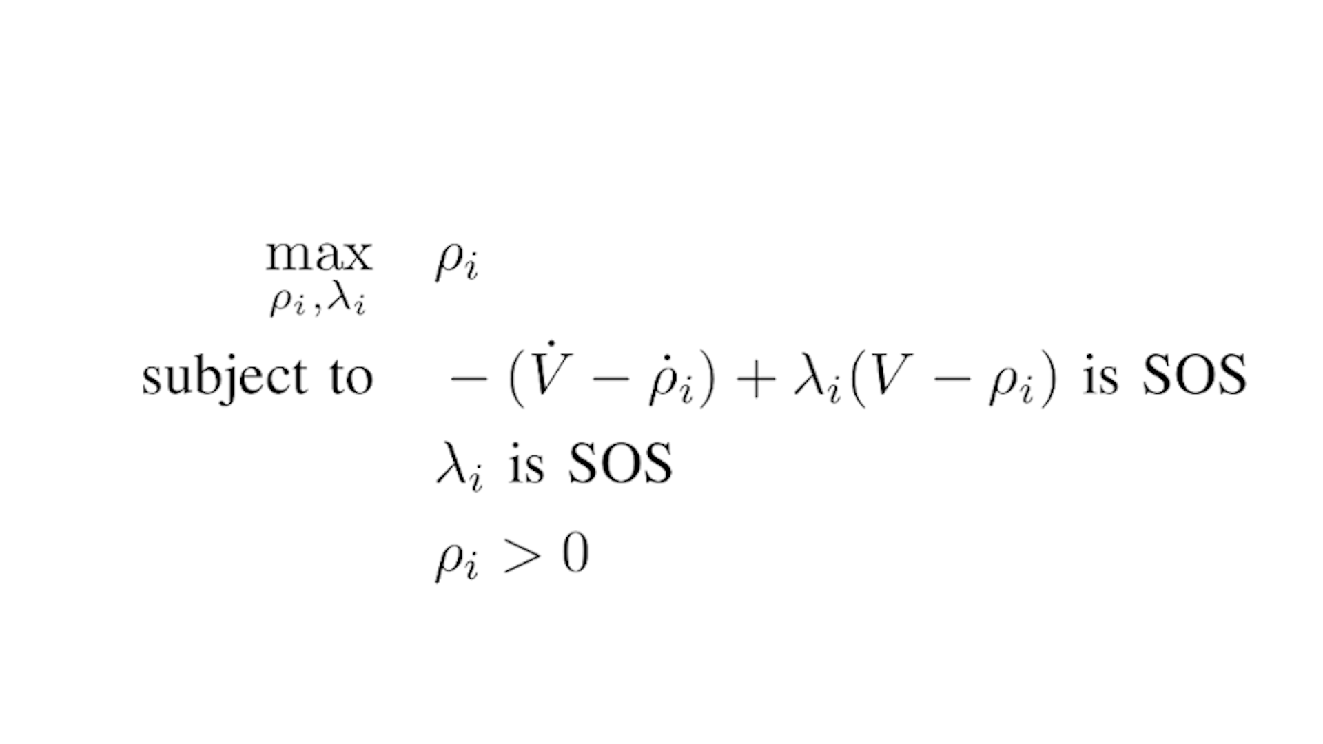
This is the optimization problem that has to be solved in order to obtain the value of rho. The Lyapunov condition has been imposed by exploiting the so-called S-procedure. Unfortunately, this formulation is not convex in rho, so that it has to be solved with a bilinear alternation by fixing at each step the Lagrangian multiplier or rho.
Furthermore, it is worthwhile to mention the consequences of considering the input saturation constraint. It can be addressed by using some Lagrangian multipliers. However, this can lead to add a number of SOS conditions that grows exponentially with the number of inputs. Hence, this has to be considered in systems where there is a big number of inputs.